QuadratiK: Collection of Methods Constructed using Kernel-Based Quadratic Distances

Introduction

QuadratiK provides a suite of methods based on kernel-based quadratic distances, and hence the name!

QuadratiK contains several goodness of Fit (GoF) tests such as normality tests and two and k-sample tests. It also includes tests for uniformity on the d-dimensional sphere, a clustering algorithm using Poisson kernel densities, and algorithms for generating random samples from PKBD. QuadratiK offers graphical functions that enhance user experience by facilitating the validation, visualization, and interpretation of clustering results. Furthermore, it provides methods for meaningful analyses and reproducible inference across diverse fields. A dashboard application with a user-friendly interface is also a part of QuadratiK to enhance accessibility for practitioners beyond the domain of statistical sciences.

This package is joint work with Dr. Marianthi Markatou, SUNY Distinguished Professor, University at Buffalo and Dr. Giovanni Saraceno, Assistant Professor, University of Padova.

Goodness-of-Fit (GoF) Tests

Goodness-of-Fit (GoF) tests are classical tools for assessing the compatibility of data with a given probability model. GoF tests typically compute a distance-like metric between the null distribution and observations, rejecting the null hypothesis if the distance exceeds a critical value.

The methods for normality, two-sample, and k-sample test use a bandwidth parameter h. We have also provided an algorithm for determining the optimal value of h based on the mid-power analysis (please see Markatou and Saraceno (2024)). You can find more details on algorithm in our manual.

In this section, the various GoF tests are shown with corresponding examples.

Normality Test

Normality tests are used to determine if the sample data is well-modeled by a normal distribution. In our case, this is done by measuring the distance between the sample data and the target distribution, where the target distribution in this case is the d-dimensional normal distribution.

In our case, this is done by measuring the distance between the empirical cumulative distribution function of the sample data and the target distribution, where the target distribution in our case is the d-dimensional normal distribution.

iimport numpy as np

np.random.seed(0)
from QuadratiK.kernel_test import KernelTest

# data generation
data_norm = np.random.multivariate_normal(mean=np.zeros(4), cov=np.eye(4), size=500)

# performing the normality test
normality_test = KernelTest(
    h=0.4, num_iter=150, method="subsampling", random_state=42
).test(data_norm)

# printing the summary for normality test
print(normality_test.summary(print_fmt="grid"))

The results of this test is shown below.

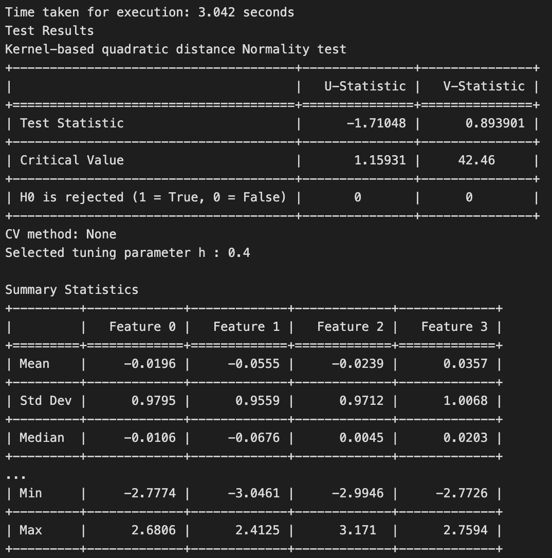
The test rightly fails to reject the null hypothesis, as the samples have been generated from a standard normal distribution.

Two-Sample Test

The two-sample GoF test is used to determine whether two separate samples are likely drawn from the same population distribution.

To illustrate the two sample test, we generate n = 200 random samples from a multivariate standard normal distribution and a skewed normal distribution with value of skewness parameter lambda = 0.1.

import numpy as np

np.random.seed(0)
from scipy.stats import skewnorm

from QuadratiK.kernel_test import KernelTest

# data generation
X_2 = np.random.multivariate_normal(mean=np.zeros(4), cov=np.eye(4), size=200)
Y_2 = skewnorm.rvs(
    size=(200, 4),
    loc=np.zeros(4),
    scale=np.ones(4),
    a=np.repeat(0.1, 4),
    random_state=20,
)
# performing the two sample test
two_sample_test = KernelTest(h=2, num_iter=150, random_state=42).test(X_2, Y_2)

# printing the summary for the two sample test
print(two_sample_test.summary(print_fmt = "grid"))

The results of the test is shown below.

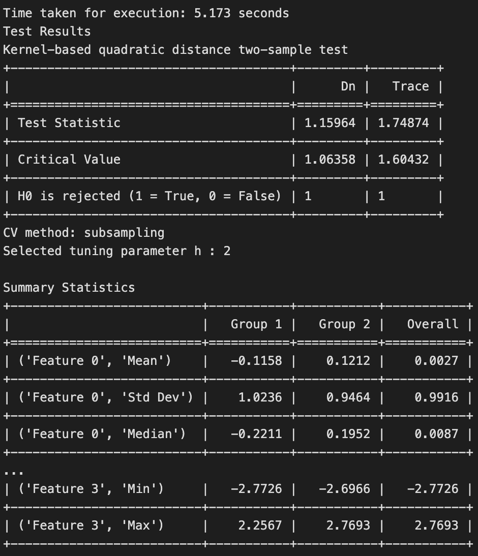
The test rejects the null hypothesis, as the samples have been generated from two different distributions.

K-Sample Test

Similar to the two-sample test, the k-sample test examines whether k groups of samples are obtained from the same distribution.

For illustrating the k-sample test, we use the glass identification dataset from the UCI ML repository. We use the first three classes of glass types to illustrate the working of the k-sample test.

# Importing required libraries
from ucimlrepo import fetch_ucirepo
import numpy as np
from QuadratiK.kernel_test import KernelTest

# Fetching the dataset
glass_identification = fetch_ucirepo(id=42)

# Selecting the data for specified types of glass
filtered_data = glass_identification.data.original.query("Type_of_glass in [1, 2, 3]")
X = filtered_data.drop(columns=['Type_of_glass'])
y = filtered_data['Type_of_glass'].to_numpy()

# Setting random seed
np.random.seed(0)

# Performing the Kernel Two-Sample Test
k_sample_test = KernelTest(h=2, num_iter=150, random_state=42).test(X, y)

# Printing the test summary
print(k_sample_test.summary(print_fmt="grid"))

The results of the test is shown below.

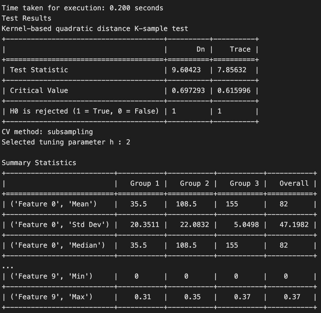
The null hypothesis is rejected for the k-sample test indicates that there is significant evidence to conclude that at least one of the distributions among the three glass types is different. In other words, the samples from the three classes of glass do not all come from the same underlying population distribution. This suggests that there are meaningful differences in the characteristics or features of the glass types being compared.

Uniformity Test on the Sphere

In this we test the null hypothesis of uniformity on the sphere. We illustrate this test using an example.

The data for this example is generated from a multivariate standard normal distribution, and is further divided by the L2 norm of generated vectors. This processed data is uniformly distributed on the surface of the unit sphere.

import numpy as np

np.random.seed(0)
from QuadratiK.poisson_kernel_test import PoissonKernelTest

# data generation
z = np.random.normal(size=(500, 3))
data_unif = z / np.sqrt(np.sum(z**2, axis=1, keepdims=True))

# performing the uniformity test
unif_test = PoissonKernelTest(rho=0.5, random_state=42).test(data_unif)

# printing the summary for uniformity test
print(unif_test.summary(print_fmt = "grid"))

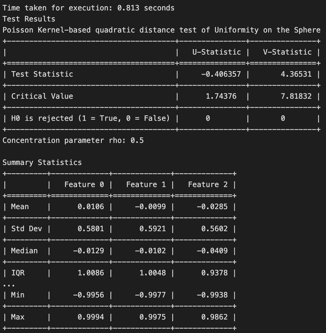
The results of the test is shown below.

Clustering

QuadratiK implements the Poisson kernel-based clustering algorithm on the sphere proposed by Golzy and Markatou (2020). We will demonstrate the spherical clustering capabilities of QuadratiK through an image segmentation task.

The image we will be using is shown below, and the task is to identify the various regions (eg. entity or other features on interest in an image).

Particularly, in this image a potential image segmentation task is to identify the various entities i.e. the cat and the dog in the image. Let’s apply the clustering algorithm and see what does it return to us.

import matplotlib.pyplot as plt
from PIL import Image
import numpy as np

# Load and resize the image
image = Image.open("dog-cat.png")
new_size = (50, 50)  # Width, Height
image = image.resize(new_size)

# Convert the image to a NumPy array
image_array_resized = np.array(image, dtype=float).reshape((-1, 3))
image_array_resized = image_array_resized + 10**-6  # Avoid division by zero

# Apply Poisson Kernel Based Clustering
from QuadratiK.spherical_clustering import PKBC

k_values = range(2, 11)
pkbc = PKBC(num_clust=k_values, random_state=0).fit(image_array_resized)

segmented_images = []

plt.figure(figsize=(16, 8))

num_k_values = len(k_values)
num_cols = 6
num_rows = (num_k_values + num_cols - 1) // num_cols

for i, k in enumerate(k_values, start=1):
    labels = pkbc.labels_[k]
    labels_reshaped = labels.reshape(new_size[1], new_size[0])

    np.random.seed(42)
    unique_labels = np.unique(labels)
    colors = np.random.randint(0, 255, size=(len(unique_labels), 3))
    segmented_image = np.zeros((new_size[1], new_size[0], 3), dtype=np.uint8)

    for label in unique_labels:
        segmented_image[labels_reshaped == label] = colors[label]

    segmented_images.append(segmented_image)

    # Plot segmented image
    plt.subplot(num_rows, num_cols, i)
    plt.imshow(segmented_image)
    plt.axis('off')
    plt.title(f"Segmented (k={k})")

plt.tight_layout()
plt.show()

The image is segmented into k clusters with k ranging from 2 to 8. Below, we display the regions identified for each value of k.

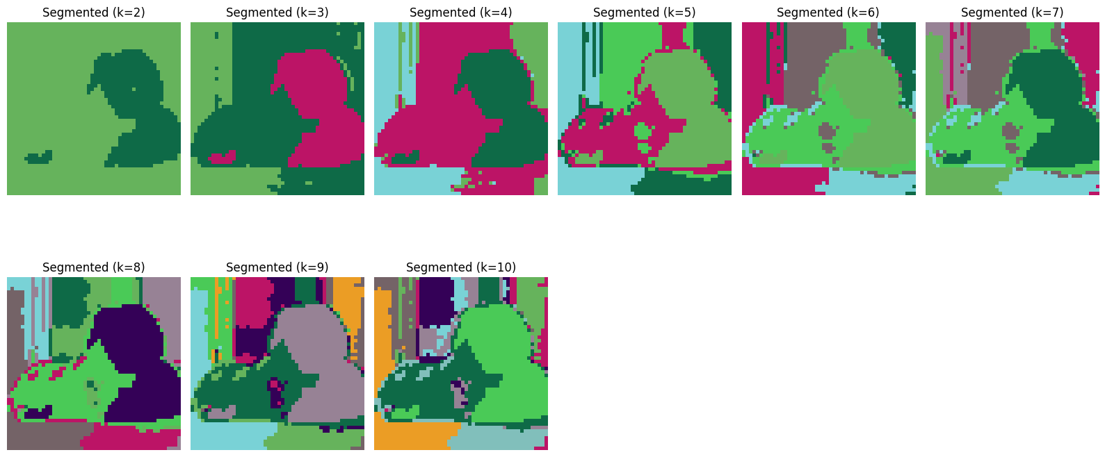
Starting from k = 5, the segmented images reveal only minor changes in the identified segments upon closer examination. Let us see if we can validate our observation using the elbow plots.

validation_metrics, elbow_plots = pkbc.validation()
elbow_plots

The elbow plots show a clear elbow at k = 5, which aligns with our observation that all regions of the image are effectively identified at this value of k.

The clustering algorithm proposed in Golzy and Markatou has been used in other works such as Golzy et al. (2023), Strelnikoff at al. (2020), and Strelnikoff et al. (2024).

Sampling from PKBD

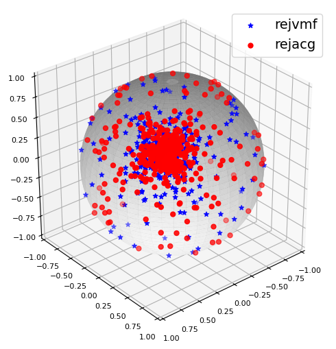
In this example, we generate observations from the Poisson kernel-based distribution on the sphere. QuadratiK in Python implements two algorithms to generate random samples, the acceptance-rejection algorithm using the Mises-Fisher and angular central Gaussian distributions. In the example, we consider mean direction $\mu = (1,1,1)$ and dimension d = 3 with concentration parameter $\rho = 0.9$. We sample n = 500 observations for the available methods.

# Import the PKBD class from the spherical_clustering module in the QuadratiK package
from QuadratiK.spherical_clustering import PKBD
# Instantiate the PKBD class
pkbd = PKBD()
# Generate 500 samples from PKBD using rejvmf
samples_rejvmf = pkbd.rpkb(
    n=500, mu=[1, 1, 1], rho=0.9, method="rejvmf", random_state=42
)
# Generate 500 samples PKBD using rejacg
samples_rejacg = pkbd.rpkb(
    n=500, mu=[1, 1, 1], rho=0.9, method="rejacg", random_state=42)

The generated samples can also be visualized on the unit sphere.

import matplotlib.pyplot as plt
import numpy as np

# Plot samples on unit sphere
phi, theta = np.mgrid[0 : np.pi : 100j, 0 : 2 * np.pi : 100j]
x = np.sin(phi) * np.cos(theta)
y = np.sin(phi) * np.sin(theta)
z = np.cos(phi)
fig = plt.figure(figsize=(5, 5))
ax = fig.add_subplot(111, projection="3d")
ax.view_init(azim=50, elev=30)
ax.plot_surface(x, y, z, color="white", alpha=0.8, linewidth=0)
ax.scatter(
    samples_rejvmf[:, 0],
    samples_rejvmf[:, 1],
    samples_rejvmf[:, 2],
    color="b",
    s=25,
    marker="*",
    label="rejvmf",
)
ax.scatter(
    samples_rejacg[:, 0],
    samples_rejacg[:, 1],
    samples_rejacg[:, 2],
    color="red",
    s=25,
    marker="o",
    label="rejacg",
)
ax.set_xlim([-1, 1])
ax.set_ylim([-1, 1])
ax.set_zlim([-1, 1])
ax.set_aspect("equal")
ax.tick_params(axis="both", labelsize=8)
plt.legend(loc="upper right", fontsize=14)
plt.tight_layout()

More details on Poisson Kernel-Based Distributions can be found in the package documentation here.

Dashboard

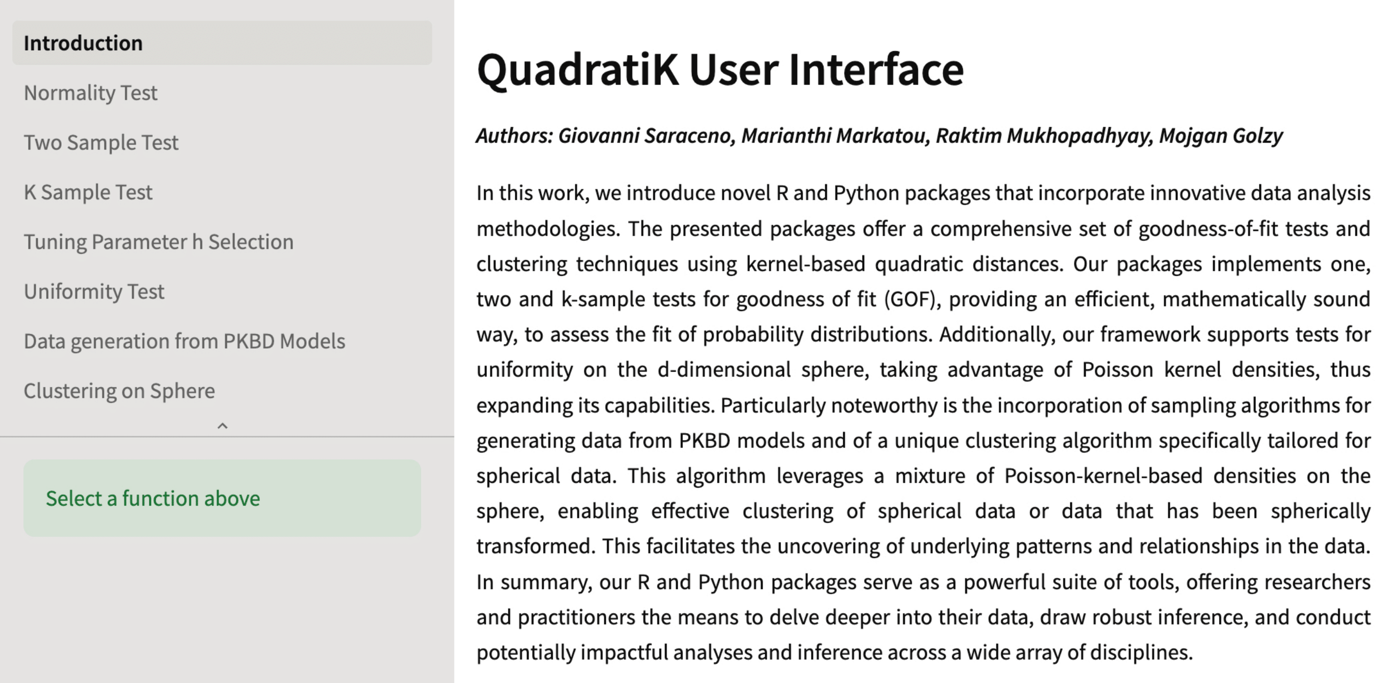
QuadratiK also provides a graphical user interface (GUI) that enables users to interact with its methods in a non-programmatic and user-friendly manner.

from QuadratiK.ui import UI
UI().run()

Concluding Remarks

QuadratiK provides methods to researchers and practitioners to delve deeper into their data, draw robust inference, and conduct potentially impactful analyses and inference across a wide array of disciplines. The QuadratiK package is also available in R and is hosted on CRAN. You can learn more about QuadratiK in our arXiv preprint. Additional theoretical papers of interest are listed in the reference section.

Please feel free to reach me at raktimmu at buffalo.edu.

Thank you! Happy coding to you — may your bugs be few, and your data ever insightful! 🚀😊

References

• Saraceno G., Markatou M., Mukhopadhyay R., Golzy M. (2024). Goodness-of-Fit and Clustering of Spherical Data: the QuadratiK package in R and Python. arXiv preprint arXiv:2402.02290.

• Ding Y., Markatou M., Saraceno G. (2023). “Poisson Kernel-Based Tests for Uniformity on the d-Dimensional Sphere.” Statistica Sinica. DOI: 10.5705/ss.202022.0347.

• Golzy M. & Markatou M. (2020) Poisson Kernel-Based Clustering on the Sphere: Convergence Properties, Identifiability, and a Method of Sampling, Journal of Computational and Graphical Statistics, 29:4, 758-770, DOI: 10.1080/10618600.2020.1740713.

• Sablica, L., Hornik, K., & Leydold, J. (2023). Efficient sampling from the PKBD distribution. Electronic Journal of Statistics, 17(2), 2180-2209.

• Markatou, M., & Saraceno, G. (2024). A unified framework for multivariate two-sample and k-sample kernel-based quadratic distance goodness-of-fit tests. DOI: 10.48550/arXiv.2407.16374v1

• Golzy, M., Rosen, G. H., Kruse, R. L., Hooshmand, K., Mehr, D. R., & Murray, K. S. (2023). Holistic assessment of quality of life predicts survival in older patients with bladder cancer. Urology, 174, 141-149.

• Strelnikoff, S., Jammalamadaka, A., & Warmsley, D. (2020, December). Causal maps for multi-document summarization. In 2020 IEEE International Conference on Big Data (Big Data) (pp. 4437-4445). IEEE.

• Strelnikoff, S., Jammalamadaka, A., & Warmsley, D. M. (2024). U.S. Patent No. 11,907,307. Washington, DC: U.S. Patent and Trademark Office.